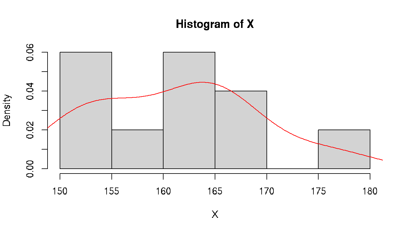
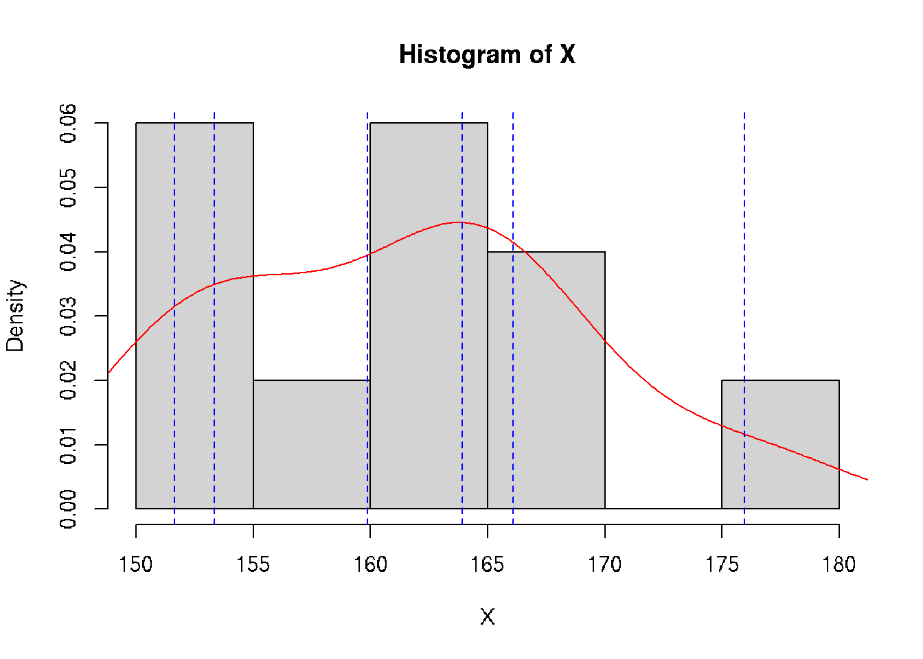
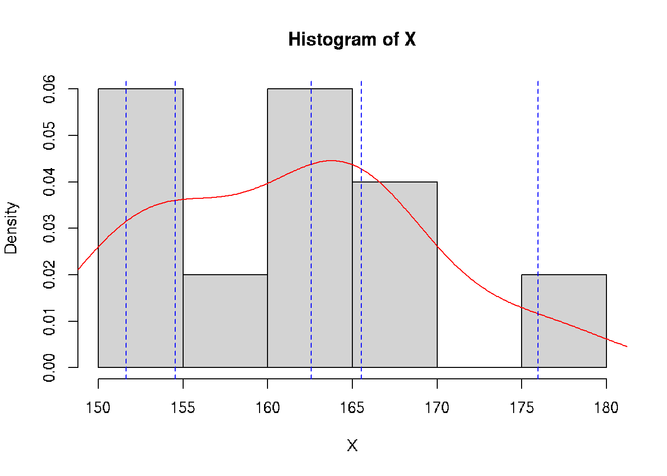
A Gentle Introduction to Biostatistics

.column.bg-main4[.vmiddle[.left[
  .font1[
.amber[Aly Lamuri]  
Indonesia Medical Education and Research Institute
  ]
]]]

---

.column.bg-white[.vmiddle.center[
{{content}}
]]

# About me
  .row[.content[
Aly Lamuri
  ]]
  .row[.content[
FKUI 2011
  ]]
  .row[.content[
Newcastle 2018
  ]]
  .row[.content[
Academic writer
  ]]
  .row[.content[
Research assistant
  ]]

]]]

---

---

---

---

---

count: false
<img src="https://upload.wikimedia.org/wikipedia/id/6/64/Makara-ui-fk.png" height="100%">

---

.column.bg-main4[.vmiddle[.font2[
- .amber[Lecture overview]
- Parameters in population
- Statistics in acquired samples
- Descriptive statistics
]]]

---

- Three hours of lecture? .red[Please, no.]
- Session: lecture, Q&A, journal discussion
- .amber[Fourteen] sessions in total
  ]]

Understand the .amber[basic] of statistics
  ]]

- Types of data and distribution
- Test of differences
- Correlation
- Simple linear model
  ]]

]]]

---

???
- Encourage active participation (+icebreaking)
- Use zoom feature: raise hand, voice chat, etc
- Kahoot!

---

---

---

# Agreement

- Attend .amber[all] lectures (at minimum: .red[80%])

--
- Be .amber[on time], even if you are late make it no longer than .red[10 minutes]

--
- Turn on the .amber[front camera] during the beginning of each lecture.

--
And smile, because I'm taking a screenshot of your attendance :)

--
- Pay .amber[attention] during classes.

--
I may randomly ask you a question

--
- .amber[Actively] participate in class

--
- You may ask for .amber[permission] to temporarily leave the class.

--
But .red[please return], because the class is gonna miss you :(

--
- Turn on the front camera during .amber[presentation]

--
- Do the .amber[assignment]

???

Show the course layout  
https://docs.google.com/document/d/1IE1H79-IQviC-vbHFSHvmMJNDbM8eiqZS69DkGHkPrY/edit?usp=sharing

---

.amber.font5[HBU?]

???
- What's your expectation in attending this biostatistics course?

---

.column.bg-main4[.vmiddle[.font2[
- Lecture overview
- .amber[Parameters in population]
- .red[Statistics in acquired samples]
- Descriptive statistics
]]]

---

## Population

<br>

## Parameters

Quantitative .amber[summary] of a population

<br>

## Be more .amber[specific,] please?

`$X$`: Data element  
`$N$`: Number of element  
`$P$`: Proportion  
`$M$`: .yellow[Median]  
`$\mu$`: .yellow[Average]  
`$\sigma$`: .yellow[Standard deviation]  
`$\sigma^2$`: .yellow[Variance]  
`$\rho$`: Correlation coefficient  
]]

---

## Sample

A .red[subset] of an observable population

<br>

## Statistics

Quantitative .red[summary] of a sample

<br>

## Be more .red[specific,] please?

`$x$`: Data element  
`$n$`: Number of element  
`$p$`: Proportion  
`$m$`: .deep-orange[Median]  
`$\bar{x}$`: .deep-orange[Average]  
`$s$`: .deep-orange[Standard deviation]  
`$s^2$`: .deep-orange[Variance]  
`$r$`: Correlation coefficient  
]]

---

.row.bg-main2[.vmiddle[
# Spot the differences!
]]

<br>

<table class=" lightable-minimal" style='font-family: "Trebuchet MS", verdana, sans-serif; width: auto !important; margin-left: auto; margin-right: auto;'>
 <thead>
  <tr>
   <th style="text-align:left;"> Statistics </th>
   <th style="text-align:left;"> Meanings </th>
   <th style="text-align:left;"> Parameters </th>
  </tr>
 </thead>
<tbody>
  <tr>
   <td style="text-align:left;"> `$x$` </td>
   <td style="text-align:left;"> Data element </td>
   <td style="text-align:left;"> `$X$` </td>
  </tr>
  <tr>
   <td style="text-align:left;"> `$n$` </td>
   <td style="text-align:left;"> Number of element </td>
   <td style="text-align:left;"> `$N$` </td>
  </tr>
  <tr>
   <td style="text-align:left;"> `$p$` </td>
   <td style="text-align:left;"> Proportion </td>
   <td style="text-align:left;"> `$P$` </td>
  </tr>
  <tr>
   <td style="text-align:left;"> `$m$` </td>
   <td style="text-align:left;"> Median </td>
   <td style="text-align:left;"> `$M$` </td>
  </tr>
  <tr>
   <td style="text-align:left;"> `$\bar{x}$` </td>
   <td style="text-align:left;"> Average </td>
   <td style="text-align:left;"> `$\mu$` </td>
  </tr>
  <tr>
   <td style="text-align:left;"> `$s$` </td>
   <td style="text-align:left;"> Standard deviation </td>
   <td style="text-align:left;"> `$\sigma$` </td>
  </tr>
  <tr>
   <td style="text-align:left;"> `$s^2$` </td>
   <td style="text-align:left;"> Variance </td>
   <td style="text-align:left;"> `$\sigma^2$` </td>
  </tr>
  <tr>
   <td style="text-align:left;"> `$r$` </td>
   <td style="text-align:left;"> Correlation coefficient </td>
   <td style="text-align:left;"> `$\rho$` </td>
  </tr>
</tbody>
</table>

]

---

.column.bg-main4[.vmiddle[.font2[
- Lecture overview
- Parameters in population
- Statistics in acquired samples
- .amber[Descriptive statistics]
]]]

---

# Data Element

- Suppose we have height data from a particular student group, denoted by `$X$`

--
- Let `$X \ni \{x_1, x_2, ..., x_n\}$`

--
- Then each of `$\{x_1, x_2, ..., x_n\}$` is the corresponding .amber[element] of the
  data

--
- .amber[Easy, right? ] Let's see some numbers.

```r
set.seed(1)
*X <- rnorm(10, mean=160, sd=10)
print(X)
```

```
##  [1] 153.7 161.8 151.6 176.0 163.3 151.8 164.9 167.4 165.8 156.9
```

```r
print(X[7])
```

```
## [1] 164.9
```

---

# Number of Element

- From previous example, we understood `$x_{1...n} \in X$`

--
- ...and each `$x$` as an element data

--
- But what about `$n$`?

--
- Turns out, `$n$` is the total number of .amber[element]!

--
- A quick demo:

```r
length(X)
```

```
## [1] 10
```

---

# Proportion

- From our synthetic data, we observed some people with a taller stature

--
- Let 165 be a threshold, where people above 165 cm considered as tall

--
- Then we can compute the .amber[proportion] of tall people compared to
  (*ahem*) not-so-tall people

--
- So, we can simply conclude: `$p = \frac{g}{n},\ where:$`  
`$p$`: Proportion  
`$g$`: Group of interest  
`$n$`: Number of element

--
- So, how many tall people do we have in our data?

```r
set.seed(1)
*X <- rnorm(10, mean=160, sd=10)
print(X)
```

```
##  [1] 153.7 161.8 151.6 176.0 163.3 151.8 164.9 167.4 165.8 156.9
```

```r
sum(X > 165) / length(X)
```

```
## [1] 0.3
```

---

# Mean

- Assume: data presents an even distribution
- Meaning that, data has a roughly **equal number of observation** on both ends
- We can calculate the .amber[average] value as a general description, with:

`$$\bar{x} = \frac{1}{n}\displaystyle \sum_{i=1}^{n} x_i$$`

---

- In action:

```r
*sum(X) / length(X)
```

```
## [1] 161.3
```

---

- In action:

```r
sum(X) / length(X)
```

```
## [1] 161.3
```

```r
*mean(X)
```

```
## [1] 161.3
```

---

- In action:

```r
sum(X) / length(X)
```

```
## [1] 161.3
```

```r
mean(X)
```

```
## [1] 161.3
```

---

On a quick glimpse:

![](index_files/figure-html/viz-1.png)

---

**Solution:** Use another measure `$\to$` median

![](index_files/figure-html/viz-1.png)

---

# Median

- Sort data ascendingly
- Find the mid point of such data
- Median is the **middle** index

--
- Or, .amber[mathematically]:

`$$m = \begin{cases} x_{\frac{n+1}{2}} & :n_{2\nmid} \\ \frac{1}{2} \left(x_{\frac{n}{2}} + x_{\frac{n}{2} + 1} \right) & :n_{2\mid} \end{cases}$$`

--
A quick demo:

```r
sort(X)
```

```
##  [1] 151.6 151.8 153.7 156.9 161.8 163.3 164.9 165.8 167.4 176.0
```

```r
median(X)
```

```
## [1] 162.6
```

```r
mean(X)
```

```
## [1] 161.3
```

---

# Standard Deviation

- In a simple term, .amber[deviation] `$d_i$` tells you how far a data element
  `$i$` is from your mean value
- So, we can calculate deviation as `$d_i = X_i - \mu$`
- **However,** the deviation can be either *negative* or *positive*

--
.row[.content[
]]

---

Take our data as an example:

```r
set.seed(1)
*X <- rnorm(10, mean=160, sd=10)
print(X)
```

```
##  [1] 153.7 161.8 151.6 176.0 163.3 151.8 164.9 167.4 165.8 156.9
```

```r
d <- X - mean(X)
print(d, digits=2)
```

```
##  [1] -7.59  0.51 -9.68 14.63  1.97 -9.53  3.55  6.06  4.44 -4.38
```

--
Hard to find its general property!

--
`$\to$` Potential solution?

---

We can take the **absolute** value and compute the mean:

`$$\bar{d} = \frac{1}{N} \displaystyle \sum_{i=1}^{N} |X_i - \mu|$$`

--
A quick demo:

```r
d <- abs(X - mean(X))
print(d, digits=2)
```

```
##  [1]  7.59  0.51  9.68 14.63  1.97  9.53  3.55  6.06  4.44  4.38
```

```r
d.bar <- mean(d)
print(d.bar, digits=2)
```

```
## [1] 6.2
```

--
Now, it's easier to report your findings as `$\bar{x} \pm \bar{d}$`

--
, or numerically as .amber[161.32] `$\pm$`
.red[6.23]

--
`$\to$` Yet, such a practice is uncommon to see.

---

Another alternative is to find the **root-mean square**, which define a
.amber[standard deviation]:

`$$\sigma = \sqrt{\frac{1}{N} \displaystyle \sum_{i=1}^N (X_i - \mu)^2}$$`

--
A quick demo:

```r
std.dev <- sqrt(sum({X - mean(X)}^2) / length(X))
print(std.dev)
```

```
## [1] 7.4
```

---

In statistics, we need to adjust the estimation by applying .amber[Bessel's correction].

--
Simply said, we find the mean by dividing into `$n-1$` instead of `$N$`.

`$$s = \sqrt{\frac{1}{n-1} \displaystyle \sum_{i=1}^n (x_i - \bar{x})^2}$$`

--
A quick demo:

```r
*std.dev <- sqrt(sum({X - mean(X)}^2) / {length(X) - 1})
print(std.dev)
```

```
## [1] 7.8
```

```r
sd(X) # Built-in function to calculate standard deviation
```

```
## [1] 7.8
```

???
Bessel's method applied to correct the bias in estimating population variance.

---

# Variance

- Another measure to estimate deviation
- Akin to standard deviation, but without a root square

--
- Computed as follow:

`$$s^2 = \frac{1}{n-1} \displaystyle \sum_{i=1}^n (x_i - \bar{x})^2$$`

--
**Importance:**

- In making further inference
- More advanced statistical model

--
(outside the scope of this lecture, sorry!)

---

# Quantile

- A .amber[cut-off] from a given probability distribution
- Divide the data into a .amber[continuous] range

**Our data:**

```r
sort(X)
```

```
##  [1] 152 152 154 157 162 163 165 166 167 176
```

---

```r
quantile(X, probs=seq(0, 1, 1/5))
```

```
##   0%  20%  40%  60%  80% 100% 
##  152  153  160  164  166  176
```
]]

---

Quartile: A special case of quantile

```r
quantile(X, probs=seq(0, 1, 1/4))
```

```
##   0%  25%  50%  75% 100% 
##  152  155  163  166  176
```
]]

---

.column[.font2.content.vmiddle[
- .amber[Central tendency:]
  - Mean
  - Median
- .amber[Spread:]
  - Standard deviation
  - Variance
  - Quantile
]]

---

.column[.vmiddle.center.content[
<img src="https://blog.optimizely.com/wp-content/uploads/2015/02/stats-cat.jpg" width="100%">
]]

---

.column.bg-white[.vmiddle.center.content[
<img src="https://i.dailymail.co.uk/i/pix/2008/09/21/article-1059095-02BF33FE00000578-967_468x482.jpg" width="100%">
]]

{{content}}
]]

---

- December **1996**, home alone with her newly born baby
- Suddenly the baby stopped responding, Sally called the ambulance
- Failed to resuscitate `$\to$` Pronounced dead, diagnosed as SIDS
- January **1998**, the same thing happened to her second child
- Post-mortem: Retro-orbital and spinal bleeding

---

- UK criminology: two infant murders in the same household is 1 in 2mil
- An extremely rare chance, indeed

---

- UK epidemiology: SIDS is about **1 in 8,500** healthy newborns
- Probability of having two consecutive cases in a row?
- Assuming independence, two consecutive cases may happen in 1:72mil
- An even rarer case!

---

.column.bg-white[.vmiddle.center.content[
<img src="https://image.freepik.com/free-photo/black-guy-blonde-woman-texting_102671-4270.jpg" width="100%">
]]

{{content}}
]]

---

- In 1964, a young lady snatched Mrs. Juanita Brooks' purse
- According to eye witnesses:
  - The culprit was a woman in mid 20s
  - Had light blond hair with a pony tail
  - Went to a yellow motor car, driven by a black American
  - The guy had beard and mustache

(**Disclaimer:** Photo is just an illustration)

---

The chance of:

- Black man with beard: **1 in 10**
- Man with mustache: **1 in 4**
- White woman with pony tail: **1 in 10**
- White woman with blond hair: **1 in 3**
- Yellow motor car: **1 in 10**
- Interracial couple in car: **1 in 1,000**

Overall probability of consecutive independent occurrence: **1 in 12mil** `$\to$`
Rare!

---

# .amber[Similarities] of both cases?

- Both relied on .amber[probability] theory.
- Basically: .amber[statistics]

--
... More or less.

--
- Used in .amber[court room] to determine innocence.

--
- ... And both were .red[**grave mistakes**].

--
- Let's quickly reinvestigate both cases :)

---

- The occurrence of SIDS is not independent
- Meaning that, there is a higher likelihood of having a second child affected
  by SIDS
- ... If your first child is
- Since they are not independent, multiplying the proportion would not do
  justice to estimate the chance

---

- Just like in Sally Clarke's case
- The chance of finding a black guy with beard and mustache... (and so on, as
  previously described)... Is not an independent event

---

# Then, is statistics .red[wrong]?

--
  .font2[
- Sometimes, we unconsciously obscure the fact with numbers
  ]

???
Example: 8 among 10 dentists recommend Colg*te

--
  .font2[
- Now we will learn some examples where statistics help telling the truth
  ]

---

# How .amber[statistics] describe .red[mental health]

.font2[
- .amber[28%] of HIV-positive participants were having .red[depressive]
  symptoms `$^1$`
- .amber[49%] of the French neurosurgical community reported .red[burnout]
  `$^2$`
- .amber[9.4%] of medical students in a study had .red[suicidal ideation]
  within the past 12 months `$^3$`
  ]

.font1[
1. S. K. Y. Choi, E. Boyle, J. Cairney, et al. .amber[“Prevalence, Recurrence, and Incidence owe Current Depressive Symptoms among People Living with HIV in Ontario, Canada: Results from the Ontario HIV Treatment Network Cohort Study”]. In: _PLOS ONE_ 11.11 (Nov. 2016). Ed.  by V. D. Lima, p. e0165816.  DOI: 10.1371/journal.pone.0165816.
1. C. Baumgarten, E. Michinov, G. Rouxel, et al. .amber[“Personal and psychosocial factors of burnout: A survey within the French neurosurgical community”]. In: _PLOS ONE_ 15.5 (May. 2020). Ed. by S. A.  Useche, p. e0233137. DOI: 10.1371/journal.pone.0233137.
1. L. N. Dyrbye, C. P. West, D. Satele, et al. .amber[“Burnout Among U.S.  Medical Students, Residents, and Early Career Physicians Relative to the General U.S. Population”]. In: _Academic Medicine_ 89.3 (Mar. 2014), pp. 443-451.  DOI: 10.1097/acm.0000000000000134.
]

---